| Brian
Harvey University of California, Berkeley |
| Download PDF version |
| Back to Table of Contents |
| BACK chapter thread NEXT |
| MIT Press web page for Computer Science Logo Style |

|
|
Program file for this chapter: plot
A particular musical note (middle C, say) played on a piano and played on a violin sound similar in some ways and different in other ways. Two different notes played on the violin also have similarities and differences. How do you hear which note is being played, and how do you know what instrument you're listening to?
To do justice to these questions would fill up an entire book. For example, a piano produces sound when a felt-covered wooden hammer hits metal wires, or strings. Each piano key controls one hammer, but each hammer may hit from one to three strings. It turns out that the strings for a particular note are not tuned to exactly the same pitch. Part of the richness of the piano's sound comes from the interplay of slightly different pitches making up the same note.
Another contributing factor to the recognition of different instruments is their differences in attack and decay. Does the sound of a note start abruptly, or gradually? The differences are not only a matter of loudness, though. A few instruments start out each note with a very pure, simple tone like a tuning fork. Gradually, the tone becomes more complex until it finally reaches the timbre you associate with the instrument. But a bowed violin, a more typical example, starts out each note almost as a burst of pure noise, as the bow hits the strings, and gradually mellows into the sound of a particular note. If you are experimentally inclined, try tape recording the same note as played by several instruments. Then cut out the beginnings and ends of the notes, and retain only the middle section. Play these to people and see how well they can identify the instruments, compared to their ability to identify the complete recorded notes.
For this chapter, though, I'm going to ignore these complications, and concentrate on the differences in the steady-state central part of a note as played by a particular instrument. What all such steady musical sounds have in common is that they are largely periodic. This means that if you graph the air pressure produced by the instrument over time (or the voltage when the sound is represented electrically in a hifi system), the same pattern of high and low pressures repeats again and again. Here is an example. In this picture, the motion of your eye from left to right represents the passing of time.
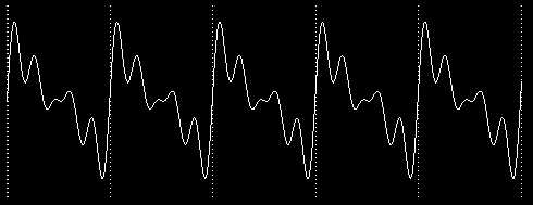
The height of the squiggle on the page, at any particular moment, represents the sound pressure at that moment. So what this picture shows is that there are many small up-and-down oscillations superimposed on one large, regular up-and-down motion. (This one large oscillation is called the fundamental frequency.) You can see that the entire picture consists of five repetitions of a smaller squiggle with just one of the large oscillations.
From what I've said about oscillations, you might get the impression that this is a picture of something like a foghorn or siren, in which you can hear an alternation of loud and soft moments. But this is actually the picture of what sounds like a perfectly steady tone. The entire width of the page represents about one one-hundredth of a second. There are a few hundred repetitions of the single large up-and-down cycle in each second of a musical note. The exact number of repetitions is the frequency of the note, and is the same for every instrument. For example, the note A above middle C has a pitch of 440 cycles per second, or 440 Hertz.
All instruments playing A above middle C will have a picture with the same fundamental frequency of 440 Hertz. What is different from one instrument to another is the exact shape of the squiggle. (By the way, the technical name for a squiggle is a waveform. You can see the waveform for a note by connecting a microphone to an oscilloscope, a device that shows the waveform on a TV-like screen.)
Here is a picture of the simplest, purest possible tone:
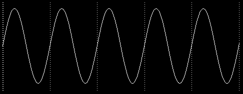
This is the waveform you'd get from an ideal tuning fork, with no impurities or bumps. It is called a sine wave. This particular kind of oscillation turns up in many situations, not just musical sounds. For example, suppose you write a program that starts a turtle moving in a circle forever.
to circle
fd 1
rt 1
circle
end
Think about the motion of the turtle, and concentrate only on its vertical position on the screen. Never mind its motion from left to right. The up-and-down part of the turtle's motion over time looks just like this sine wave.
This says more than simply that the turtle alternates moving up and down. For example, the turtle's vertical motion might have looked like this over time:
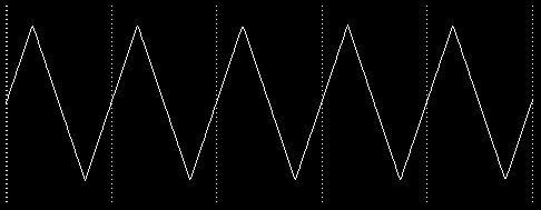
If this were the picture of the turtle's motion, it would mean that the turtle's vertical position climbed at a steady rate until it reached the top of the circle, then abruptly turned around and started down again. But in fact what happens is that the height of the turtle changes most quickly when the turtle is near the "Equator" of its circle. The turtle's vertical speed gets less and less as the turtle gets near the "poles." This speed change corresponds to the gradual flattening of the sine wave near the top and bottom. (You may find it confusing when I say that the turtle's vertical motion slows down, because the turtle's speed doesn't seem to change as it draws. But what happens is that near the Equator, the turtle's speed is mostly vertical; near the poles, its speed is mostly horizontal. We aren't thinking about the horizontal aspect of its motion right now.)
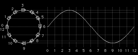
What makes sine waves most important, though, is that any periodic waveform can be analyzed as the sum of a bunch of sine waves of different frequencies. (Sometimes an infinite number of since waves must be added together.) The frequencies of the sine waves will always be multiples of the fundamental frequency. This important mathematical result was discovered by the French mathematician Jean-Baptiste-Joseph Fourier (1768-1830). The representation of a mathematical function as a sum of sine waves is called a Fourier series.
For example, when a violin plays A above middle C, the waveform that results will include a sine wave with frequency 440 Hertz, one with frequency 880 Hertz, one at 1320 Hertz, and so on. Not all of these contribute equally to the complete waveform. The amplitude of each sine wave (the amount of swing, or the vertical distance in the picture) will be different for each. Typically, the fundamental frequency has the largest amplitude, and the others (which are called harmonics or overtones) have smaller amplitudes. The precise amplitudes of each harmonic are what determine the steady-state timbre of a particular instrument.
Two traditional musical instruments, the clarinet and the pipe organ, share a curious characteristic: their Fourier series contain only odd harmonics. In other words, if a clarinet is playing A above middle C, the waveform includes frequencies of 440 Hertz, 1320 Hertz (3 times 440), 2200 Hertz (5 times 440), and so on. But the waveform does not include frequencies of 880 Hertz (2 times 440), 1760 Hertz (4 times 440), and so on. (I'm oversimplifying a bit in the case of the pipe organ. What I've said about only odd harmonics is true about each pipe, but the organ can be set up to combine several pipes in order to include even harmonics of a note.)
In recent times, a third musical instrument has come to share this peculiar Fourier series: the computer. (Perhaps you were wondering where computers come into this.) Today there are computer-controlled musical instruments that can generate any possible sound. Musicians have even used computers to create new instrument timbres that are not possible with ordinary instruments. But the particular timbre that most people associate with computer music is the one produced by the simplest possible computer sound generator. Instead of a steady oscillation in sound pressure, this simple device can only be on or off at a given moment. The computer produces sound by flipping the device from on to off and back at a particular rate. Such a device produces a square wave, like this:

No sound that occurs in nature has a waveform that turns corners so abruptly. But what is "natural" in nature isn't necessarily what's "natural" for a computer. For many years, computer-generated music invariably meant square waves except in very fancy music research centers.
More recently, new integrated circuit technology has made it relatively inexpensive to equip computers with "music chips" that generate sine waves. The stereotyped sound of computer music is becoming uncommon. But I still find square waves fascinating for several reasons.
One place where square waves are still used is in the hifi magazines, in their tests of amplifiers. The testing laboratories feed a square wave into an amplifier, and show oscilloscope pictures of the waveform going into the amp and the waveform coming out. Here is an example:
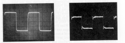
The oscillation that is visible in the output near the corners of the input is called ringing. A lot of ringing indicates that the amplifier doesn't have good high-frequency response.
Here is why a square wave is a good test of high frequencies: The Fourier series corresponding to the square wave includes an infinite number of odd-harmonic sine wave components. In other words, a perfect square wave includes infinitely high frequencies. (In practice, the input picture isn't a perfect square wave. You can see that the vertical segments aren't quite truly vertical, for example.) No amplifier can reproduce infinitely high frequencies faithfully. The result is that the output from the amplifier includes only some of the harmonics that make up the input. It turns out that such a partial series, with relatively few of the harmonics included, produces a waveform in which the ringing phenomenon at the corners is clearly visible.
If you think about it, that's a bit unexpected. Normally, the more harmonics, the more complicated the waveform. For example, the simplest waveform is the one with only the fundamental, and no added harmonics. Yet, removing harmonics from the square wave produces a more complicated picture. I like paradoxes like that. I wanted to write a computer program to help me understand this one.
Before you can look into the square wave in detail, you have to know not only the fact that it uses odd harmonics, but also the amplitude of each harmonic. A square wave with fundamental frequency f has this formula:

The dots at the end indicate that this series goes on forever. The amplitude of each sine wave is the reciprocal of the harmonic number (one divided by the number).
This project draws pictures of waveforms containing some number of terms of this series. (Each sine wave is called a term.) The program allows many different ways of controlling exactly what is drawn.
To start with something very simple, try this instruction:
plot 1
The effect of this command is to draw one cycle of a pure sine wave:
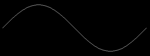
This is the first term of the series for the square wave. Now try this:
plot 5
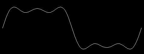
The
input to plot is the harmonic number of the highest harmonic.
In this example, we've drawn three sine waves added together: the
fundamental, third harmonic, and fifth harmonic.
To see a plot looking somewhat more like the pictures in the amplifier tests, try
plot 23
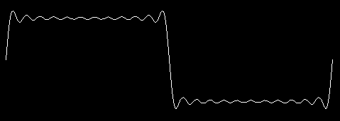
This contains the first 12 odd harmonics. (Remember to use an odd number as input, if you want to see something that looks like a square wave.) You can see that the result still includes some oscillation in the horizontal sections, but does have an overall square shape.
A mediocre hifi amp has a frequency response that is good to about 20,000 Hertz. This is about the 45th harmonic of 440 Hertz. To see how A above middle C would come out on such an amplifier, try
plot 45
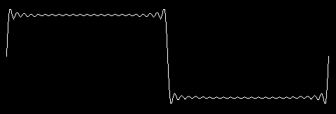
There is still some ringing near the corners, but the middle of the horizontal segment is starting to look really flat. A better amplifier might be good to 30,000 Hertz. To see how that would look, try
plot 77

(The
drawing of the picture takes longer when you use a larger input
to plot, because the program has to calculate more terms of the series.)
So far, we have only changed one of the possible parameters controlling the waveform, namely the highest harmonic. The program allows you to control several other elements of the picture. For example, try this:
plot [maxharm 77 yscale 140 deltax 1]
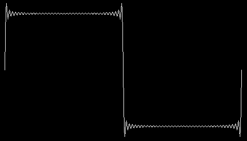
Plot takes one input, but this time the input is a list instead of
a single number. The members of the list are used as sort of "sub-inputs."
The odd-numbered members are the names of parameters,
for which the even-numbered members provide values.
Maxharm stands for "maximum harmonic"; it is the parameter you were
setting when you used a single number as the input. Yscale is an
adjustment for the height of the plot. (To "scale" a bunch of numbers
means to multiply all of them by some constant value, the "scale factor.")
You may have noticed that as the
number of harmonics has increased, the pictures have been getting smaller in
the vertical direction; by increasing the value of yscale we can
expand the height of the plot to show more detail. Similarly, deltax
allows us to show more horizontal detail, not by widening the picture but by
computing the value for every dot. Ordinarily, the program saves time by
calculating every second dot. This approximation is usually good enough,
but sometimes not. (Deltax means "change in X." Delta is the
name of the Greek letter D (Δ), which mathematicians use to represent
a small change in something.)
Here's another example:
plot [11 cycles 5]
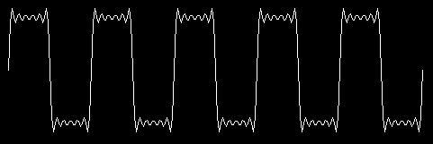
Cycles indicates
the number of complete cycles you want to see. By saying cycles 5
in this example, I drew a picture like the ones near the beginning
of this chapter, with five repetitions of the fundamental oscillation.
Notice also that we didn't have to say maxharm. If a number
appears in the input list where a name should be, it's automatically assigned
to maxharm.
Plot allows you to specify any of six parameters. Each parameter
has a default value, the value that is used if you don't say
anything about it. For example, the default value for deltax is 2.
Here are all the parameters:
| name | default | purpose |
|---|---|---|
| maxharm | 5 | highest harmonic number included in series |
| deltax | 2 | number of turtle steps skipped between calculations |
| yscale | 75 | vertical motion is multiplied by this number |
| cycles | 1 | number of cycles of fundamental shown |
| xrange | 230 | highest X coordinate allowed |
| skip | 2 | number of harmonics skipped between terms |
You've already seen what maxharm, yscale, deltax,
and cycles are
for. Now I'll explain the others.
Xrange is mainly changed when moving the program from
one computer to another. Each computer allows a particular number
of turtle steps to fit on the screen in each dimension, horizontal
and vertical. Xrange is the largest horizontal position plot
is allowed
to use. This is set a little below the largest possible X coordinate,
just to make sure that there is no problem with wrapping around the
screen.
Skip is the number of harmonics skipped between terms. To get odd
harmonics, which we need for the square wave, we have to skip by 2
each time, from 1 to 3, from 3 to 5, and so on. Different values
for skip will give very different shapes.
For example, if you are at all adventurous, you must have tried an
even value of maxharm a while ago, getting a result like this:
plot 6

What you see is two cycles of an approximation to another shape, the sawtooth:
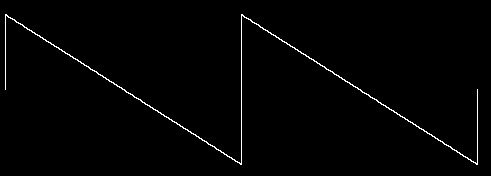
Why
two cycles? Well, plot 6 uses the
second, fourth, and sixth harmonics.
Supposing that the fundamental frequency is 440 again, this means
that plot added frequencies of 880, 1760, and 2640 Hertz. But these
are also the fundamental, second harmonic, and third harmonic of 880
Hertz. By choosing only even harmonics, you've essentially chosen
all the harmonics of twice the fundamental frequency you
had in mind. It is this doubling of the fundamental frequency that
produces two cycles on the screen. You could get one cycle of the
same waveform by saying plot [3 skip 1]:
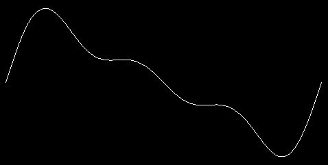
You can see much more bizarre waveforms by using other values of skip.
The best one I've found is plot [16 skip 3]:
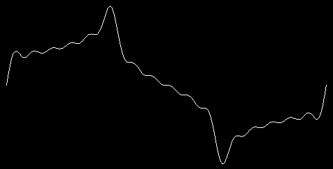
I
chose a maxharm of 16 because it includes the fundamental plus five
additional harmonics (4, 7, 10, 13, 16). If I'd made maxharm 15 or
17, I wouldn't have included the fundamental.
There are two different points of interest about this project. One
is the whole business of waveforms and Fourier series. The second
is the use of keyword inputs, which is the name for this system
of giving information to plot. The more usual style of Logo programming
would have been to make plot a procedure with six inputs. To draw
a default graph, you would then have had to say
plot 5 2 75 1 230 2
Since most of the time you want to use the default values for most of the inputs, all this typing would be an annoyance. It would also be easy to make a mistake about the correct order of the inputs. (This more usual Logo technique is called positional inputs.) The combination of many necessary inputs with standard values for most of them makes the keyword technique appropriate here. It isn't always appropriate. You wouldn't want to have to say
print item [index 2 list [vanilla chocolate strawberry]]
because you have no trouble remembering which input to item
is which, and you always want to provide both of them.
The procedure that interprets the keyword inputs is called keyword.
Keyword was written to be a general tool, not limited to this particular
program. It takes two inputs. The first is the input that you,
the user, provide. The second is a list of defaults. When plot invokes
keyword, the second input is this:
[maxharm 5 deltax 2 yscale 75 cycles 1 xrange 230 skip 2]
This input tells keyword the names of all the keyword inputs
as well as their default values. It's in the same form as the actual
input you give (a list of alternating names and values), and in fact
keyword uses a single subprocedure, first to process the default list
and then to process your input.
Keyword is actually not perfectly general because it uses the
assumption that all the values it gets are numeric. The virtue of this
assumption is that it allows keyword to recognize a number without a
name as implicitly referring to the maxharm keyword. (The name
maxharm is not built into the procedure. Instead, the first name in the
list of default values is used.) To use keyword in a context in which
non-numeric words could be values as well as names, this assumption would
have to be removed.
I didn't have keyword inputs in mind from the beginning. When I started
working on this project, the only input to plot was what I now call
maxharm, the highest harmonic number to include. All the other numbers
were "wired in"; if I wanted to change something like what is now
called :xrange, I'd edit all the procedures and change the numbers
in the editor.
Editing all the procedures wasn't too difficult, since without the
keyword-processing procedures everything fits in a single screenful.
Changing the resolution (what is now :deltax) was a bit annoying,
since I had to edit three different parts of the program. (You can
see that :deltax appears three times in the final version.) When
I finally got tired of that editing process, I decided to use keyword
inputs.
The job of keyword is to create variables, one for each keyword,
and assign a value to each variable. If the user provides a value for
a particular keyword, that's the value to use; if not, the default
value is used.
When I first did this project, I wrote a version of keyword that
creates global variables for the keywords:
to keyword :inputs :defaults
if or (wordp :inputs) (numberp first :inputs) ~
   [make "inputs sentence (first :defaults) :inputs]
setup.values :defaults
setup.values :inputs
end

to setup.values :list
if emptyp :list [stop]
make first :list first butfirst :list
setup.values butfirst butfirst :list
end
Keyword checks for the special cases of a single number
(as in plot 5) or a list beginning with a number; in either case,
a new list is made with the first keyword (maxharm) inserted before
the number. Then the default values are assigned to all the keyword
variables, and finally the user's values are assigned to whatever keywords
the user provided, replacing the defaults.
Since these keyword variables are only used within the plot program,
it would be cleaner to make them local to plot, just as ordinary
positional inputs are automatically local to a procedure. I could have
had plot take care of this before calling keyword:
to plot :inputs
local [maxharm deltax yscale cycles xrange skip]
keyword :inputs [maxharm 5 deltax 2 yscale 75 cycles 1 xrange 230 skip 2]
...
but I thought it would be unaesthetic to have to type the
names twice! What I really want is for keyword to be able to
make the variables local. But I can't just say
to keyword :inputs :defaults
local filter [not numberp ?] :defaults
if or (wordp :inputs) (numberp first :inputs) ~
   [make "inputs sentence (first :defaults) :inputs]
setup.values :defaults
setup.values :inputs
end
because that would make the variables local to keyword
itself, not to its caller, plot. This is the same problem I had
in writing localmake in Chapter 12, and the solution is the
same: Make keyword a macro!
.macro keyword :inputs :defaults
if or (wordp :inputs) (numberp first :inputs) ~
   [make "inputs sentence (first :defaults) :inputs]
output `[local ,[filter [not numberp ?] :defaults]
         setup.values ,[:defaults]
         setup.values ,[:inputs]]
end
Now it will be plot, instead of keyword, that creates the
local variables and calls setup.values.
The actual assignment of values to the keywords is a good illustration of indirect assignment in Logo. The instruction that does the assignment is this:
make first :list first butfirst :list
Usually the first input to make is an explicit quoted word,
but in this program the variable names are computed, not explicit.
This technique would be impossible in most programming languages.
It's important that the program computes the Fourier series starting with the higher harmonic numbers, adding in the fundamental term last. Recall the formula for the series:

The value of the sine function for each term is divided by the harmonic number of the term. In general, this means that the terms for higher numbered harmonics contribute smaller values to the sum.
Theoretically, it shouldn't matter in what order you add up a bunch of numbers. But computers carry out numeric computations with only a limited precision. Usually there is a particular number of significant digits that the computer can handle. It doesn't matter how big or small the number is. The numbers 1234, 1.234, and 0.00000001234 all have four significant digits.
To take a slightly oversimplified case, suppose your computer can handle six significant digits. Suppose that the value of the fundamental term is exactly 1. Then the computer could add 0.00001 to that 1 and get 1.00001 as the result. But if you tried to add 0.000001 to 1, the result (1.000001) would require seven significant digits. The computer would round this off to exactly 1.
Now suppose that the 23rd term in some series is 0.000004, the 24th term is 0.000003, and the 25th is 0.000002. (I just made up these values, but the general idea that they'd be quite small is true.) Suppose we are adding the terms from left to right in the formula, and the sum of the first 22 terms is 2.73. Adding the 23rd term would make it 2.730004, which is too many significant digits. This sum would be rounded off to 2.73 again. Similarly, the 24th and 25th terms would make absolutely no difference to the result.
But now suppose we add up the terms from right to left. The sum of the 25th and 24th terms is 0.000005, and adding in the 23rd term give 0.000009. If we were to add this to 2.73 the result would be 2.730009. Although this is still too many significant digits, the computer would round it off to 2.73001. The three terms at the end would make a small difference in the result.
In the square wave series, the successive terms get smaller quite slowly. You'd have to add very many terms before the problem I'm describing would really be important. But other series have terms that get smaller quickly, so that even for a small number of terms it's important to add in the smaller terms before the larger ones.
By the way, the procedure series that computes the value of the
series for some particular x value is written recursively, but
its task is iterative. I could have said
to series
localmake "result 0
for [harmonic :maxharm 1 [-:skip]] ~
    [make "result :result + (term :harmonic)]
output :result
end
but the use of make to change the value of a variable
repeatedly isn't very good Logo style. What I really want is an
operation corresponding to for, analogous to map as the
operation corresponding to foreach. Then I could say
to series
output accumulate "sum [harmonic :maxharm 1 [-:skip]] [term :harmonic]
end
You might enjoy using the techniques of Chapter 10 to
implement accumulate.
One final point about the programming style of this project has to do with the use of Logo's dynamic scope. Every procedure has access to the variables of its superprocedures, and this project takes advantage of the fact. Many people think it's better style if every procedure is given all the information it needs as inputs. I didn't follow that rule in this project because, as I've said, many of the variables were invented late in the development process, and I did as little rewriting as possible.
For example, here is the procedure that computes one term of the Fourier series:
to term :harmonic
output (sin :xscale * :harmonic * :x) / :harmonic
end
Of the three numbers that are used in this computation,
:xscale is constant throughout the program, so it's not unreasonable for it
to be used globally. But :x changes for every point. X is, in
fact, a local variable, but it's local to plot rather than to
term.
Why does it matter? One reason is that people find it easier to understand
a program if it's made very clear where each variable gets its value. In
this example, it's easy to miss the fact that x is the index variable
in a for loop. The second reason is that as written, term can
be used only within plot. If we wanted to compute the value of a
Fourier series for some reason other than plotting it, we couldn't easily
use the same procedures.
I decided to leave the program as it is, instead of cleaning it up for publication, so that you could see an example of a style that, after all, Logo makes possible by choosing to use dynamic scope. In some ways, this style is simpler than one in which each procedure would have several more inputs. You can decide for yourself if you find it easier or harder to read the program this way, compared to the officially approved style:
to term :x :harmonic :xscale
output (sin :xscale * :harmonic * :x) / :harmonic
end
In this version of the procedure, I've made x the first
input to term. This seems most natural to me, considering that
term's job is to compute an algebraic function of x. The argument to
a function is very naturally represented in a computer program as
the input to a procedure.
All I've changed in term itself is the title line. But of course
the invocation of term, which is in the procedure series, must
be changed also. And to be consistent, series should get its
needed values as explicit inputs, too:
to series :x :harmonic :skip :xscale
if :harmonic < 1 [output 0]
output (term :harmonic)+(series :harmonic-:skip)
end
We're up to four inputs, and it'd be easy to get them out of
order when series is invoked by plot. You can see why
"inheriting" variables from a procedure's caller can simplify its use.
The fact that each term in the series is divided by :harmonic limits this
program to a particular family of waveforms, the family that includes
square waves and sawtooth waves. In general, real musical instruments
don't have such regularity in the extent to which each term contributes
to the sum. For example, I started
by saying that clarinets and pipe
organs are made of odd harmonics, just as square waves are. But clarinets
don't sound like organs, and neither sound like square waves. There
is a family resemblance, but there are definite differences too.
The differences are due to the different "weights" that each instrument
gives to each harmonic.
Instead of the maxharm and skip
variables in the program as I've written
it, you could have an input called timbre (a French word for
the characteristic sound of an instrument, pronounced sort of like
"tamper" with a B instead of the P) that would be a list of
weighting factors. The equivalent of plot 5 would be this timbre
list:
[1 0 0.3333 0 0.2]
This list says that the fundamental has a weight of 1, the second harmonic has a weight of 0 (so it's not used at all), the third harmonic has a weight of 1/3, and so on.
The timbre version of the program would be perfectly general. You
could create any instrument, if you could find the right weighting
factors. But so much generality makes it hard to know where to begin
exploring all the possibilities. Another thing you could do would
be to try different kinds of formulas for weighting factors. For
example, you could write this new version of term:
to term :harmonic
op (sin :xscale * :harmonic * :x)/(:harmonic * :harmonic)
end
What waveforms would result from this change?
If you're really interested in computer-generated music, you'll want to hear what these waveforms sound like. Unfortunately, it's hard to do that with the standard sound generators in personal computers, which allow little or no control of timbre. But if you have one of the computer-controllable musical instruments that have become available recently, you may be able to program them to reproduce the timbre of your choice.
On the other hand, you can hear the effect of different waveforms without a computer if you visit the Exploratorium in San Francisco, the world's best museum. Among their exhibits are several that let you experiment with different ways of generating sounds. One of these exhibits is a machine that does audibly the same thing we've been doing graphically, adding up selected harmonics of a fundamental pitch. If you don't live near San Francisco, the Exploratorium is well worth the trip, no matter how far away you are!
| (back to Table of Contents) | BACK chapter thread NEXT |
As mentioned in the text, the appropriate value of xrange may be
different depending on which computer you're using.
to plot :inputs
keyword :inputs ~
        [maxharm 5 deltax 2 yscale 75 cycles 1 xrange 230 skip 2]
localmake "xscale :cycles*180/:xrange
splitscreen clearscreen hideturtle penup
setpos list (-:xrange) 0
pendown
for [x :deltax [2*:xrange] :deltax] ~
    [setpos list (xcor+:deltax) (:yscale * series :maxharm)]
end

;; Compute the Fourier series values

to series :harmonic
if :harmonic < 1 [output 0]
output (term :harmonic)+(series :harmonic-:skip)
end

to term :harmonic
output (sin :xscale * :harmonic * :x) / :harmonic
end

;; Handle keyword inputs

.macro keyword :inputs :defaults
if or (wordp :inputs) (numberp first :inputs) ~
   [make "inputs sentence (first :defaults) :inputs]
output `[local ,[filter [not numberp ?] :defaults]
         setup.values ,[:defaults]
         setup.values ,[:inputs]]
end

to setup.values :list
if emptyp :list [stop]
make first :list first butfirst :list
setup.values butfirst butfirst :list
end
Brian Harvey,
bh@cs.berkeley.edu