| Brian
Harvey University of California, Berkeley |
| Download PDF version |
| Back to Table of Contents |
| BACK chapter thread NEXT |
| MIT Press web page for Computer Science Logo Style |

|
|
Program file for this chapter: fsm
As I explained in the preface to the first volume, one of my purposes in writing this series of books has been to urge computer hobbyists away from the view of computer expertise as the knowledge of obscure characteristics of some particular computer--how to program it in machine language, what magic numbers can be found where in its memory, how to overcome the copy protection schemes on its disks, and so on. The trouble with this sort of machine-specific expertise is that it becomes obsolete when your favorite computer does. From my point of view, one of the virtues of Logo as a programming language is that its high level data structures direct your attention away from questions about what goes where in memory, allowing you to focus instead on a more abstract description of your problem.
Automata theory is a further step in abstracting your attention away from any particular kind of computer or particular programming language. In automata theory we consider a mathematical model of computing. Such a model strips the computational machinery--the "programming language"--down to the bare minimum, so that it's easy to manipulate these theoretical machines (there are several such models, for different purposes, as you'll soon see) mathematically to prove things about their capabilities. For the most part, these mathematical models are not used for practical programming problems. Real programming languages are much more convenient to use. But the very flexibility that makes real languages easier to use also makes them harder to talk about in a formal way. The stripped-down theoretical machines are designed to be examined mathematically.
What's a mathematical model? You'll see one shortly, called a "finite-state machine."
The point of this study is that the mathematical models are, in some important ways, equivalent to real computers and real programming languages. What this means is that any problem that can be solved on a real computer can be solved using these models, and vice versa. Anything we can prove about the models sheds light on the real problems of computer programming as well.
The questions asked in automata theory include these: Are there any problems that no computer can solve, no matter how much time and memory it has? Is it possible to prove that a particular computer program will actually solve a particular problem? If a computer can use two different external storage devices (disks or tapes) at the same time, does that extend the range of problems it can solve compared to a machine with only one such device?
There is also a larger question lurking in the background of automata theory: Does the human mind solve problems in the same way that a computer does? Are people subject to the same limitations as computers? Automata theory does not actually answer this question, but the insights of automata theory can be helpful in trying to work out an answer. We'll have more to say about this in the chapter on artificial intelligence.
What kinds of problems can we give to our abstract computers? In automata theory we want to focus our attention on computation itself, not on details of input and output devices. So we won't try creating a mathematical model of a video game.
We will play a game, though. In this game the computer has a rule in mind.
You type in strings of letters, using only the letters A, B, and
C. The computer tells you whether each string follows the rule or
not. Your job is to guess the rule. For example, suppose you have done
these experiments:
| accepted | rejected |
|---|---|
ABC | CBA
|
AAA | BBB
|
ABCABCABC | BCABCABC
|
A | BBBBBBB
|
ACCCCCCCCC | CAAAAAAAAA
|
You might guess, from these examples, that the rule is
"The string must begin with A." Once you've made a guess you can
test it out by trying more examples.
The program to play the game is called game. It takes one input,
a number from 1 to 10. I've provided ten different rules. Rules 1 to 3
should be pretty easy to guess; rules 8 to 10 should be nearly impossible.
(Don't feel too frustrated if you don't get them.)
A string can be any length, including length zero (the empty string). Each
time you type a letter the program lets you know whether the string you've
typed so far obeys the rule. The program indicates whether the string is
accepted or rejected by displaying the word accept or reject on
the screen. In particular, as soon
as you start game the program will tell you whether or not the empty
string is accepted by this rule. If you type the string ABC you'll
really be testing three strings: A, AB, and ABC. You
should type one letter at a time to make sure the program has a chance to
respond to it before going on to the next letter. To start over again with
a different string, press the Return key.
You should stop reading now and try the game. In the following paragraphs I'm going to talk about some of the answers, so this is your last chance. After you've figured out at least some of the rules, come back to the book.
The point of studying this game is that we're going to look at a way to design a special-purpose abstract computer that understands one particular rule. We can then ask questions about how much information the computer needs to handle the job.
You've seen the word state before in connection with the Logo
turtle. Its state includes its position and its heading. So one turtle
state might be "position [17 82], heading 90." In principle,
the turtle has an infinite number of possible states, because its
position and heading don't have to be integers. Its position might be
[14.142 14.142], for instance.
Anything that holds information can be in different states. As another example, an on-off light switch has two states. Some lamps have four states: off, low, medium, and high. A computer, too, has a certain number of states. The state of a computer includes all the information in its memory at some particular time.
A machine that has only a limited number of states, like the example of the light switch, is called a finite-state machine. For almost all of this chapter we'll be dealing with finite-state machines. You might think that that imposes a very severe limit on the kinds of computations we can do. But note that in the game I asked you to play, a rule can accept an infinite number of possible strings and reject an infinite number of others. The accepted or rejected strings can be of any length. (Some rules restrict the length of a string, but others allow any length at all.) In some sense, a finite-state machine can still perform infinitely varied computations.
Consider the third game as an example. The rule is "Accept
any string that starts with AB." Here is a picture of a finite-state
machine that implements that rule:

Each numbered circle represents a state. This machine has three
states. The start arrow indicates that the machine starts out in state
1. State 3 is shown with a double circle to indicate that it is an
accepting state. In other words, when the machine is in state 3 the
screen says accept. The other two states are not
accepting states.
Every time you type a character the machine switches from one state to
another. The arrow from state 1 to state 2 has an A next to its
tail. This indicates that when the machine is in state 1, an input of
A switches it to state 2. (The arrow from state 3 to itself has the
three letters ABC at its tail. This is a shorthand notation for
three separate arrows with heads and tails in the same place, one for each
letter.)
This picture is actually incomplete. For a full description of the machine
we have to indicate what happens on any input in any state. In other words,
each circle should have three arrows coming out from it, one each
for A, B, and C. I've chosen to adopt the convention that
every machine has an unmarked state called reject. Any missing arrow
goes to that state; once the machine is in the reject state it stays
there forever. Here, then, is the complete diagram of the machine for game
3:
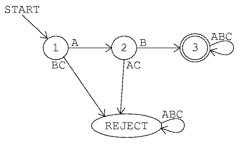
From now on I won't draw the reject state, but you should
remember that it's really part of the machine description. So this machine
requires four states, not three.
If the first input letter isn't A, the machine goes to the reject
state. If the first letter is A, the machine goes to state 2. Then,
if the second letter is B, the machine ends up in state 3 and accepts
the string AB. This is the shortest acceptable string.
Each of the three arrows from state 3 loops right back into state
3 itself. (Remember, although only one arrow appears in the picture,
it is labeled with three letters, so officially it represents three
arrows.) This means that once the machine is in state 3 it stays
there no matter what inputs it gets. Any string that starts AB is
acceptable.
Here is a machine for game number 2:
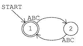
In this machine the start state is also an accepting
state. (Every machine has exactly one start state, but it may have any
number of accepting states.) This machine never gets into the reject
state. That doesn't mean it doesn't reject any strings; all odd-length
strings are rejected in state 2. But a rejected string can redeem itself by
adding another input character, so state 2 allows a return to the accepting
state 1.
Here is a machine for game number 5. (Notice that I'm saying "a machine" and not "the machine"; it is always possible to design other machines that would follow the same rule.)
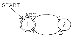
You probably had more trouble discovering rule 5 than rule
2, and it takes longer to say the rule in English words. But the
machines for the two rules are almost identical. (Remember,
though, that the rule-5 machine really has a third state, the reject
state, which is not shown in the diagram.)
Here are machines for rules 7 and 9. With these machines as hints,
can you figure out the rules? Go back to the game program to test
your hypotheses.

You should also get some practice translating in the other direction, from
English rules to machine diagrams. Here are a couple to work on: Rule 4 is
"To be accepted a string must be composed of doubled letters (AA,
BB, and CC) strung together." Rule 8 is "To be accepted a
string must contain an even number of As."
Here is rule 6: "To be accepted a string must begin with A and end
with C." Strings accepted by this rule include AC (the shortest
possible), ABC, AACC, ACAC, ABCABC, and so on.
Between the initial A and the final C an accepted string can
have any combination of As, Bs, and Cs. It's natural to
think of the string as having three parts: a fixed beginning, a variable
middle, and a fixed end. The three parts of the input strings can be
represented conveniently with three states in the machine, like this:
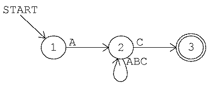
The machine starts in state 1. To be accepted a string must start
with A. Therefore, an A arrow leads from state 1 to state 2. Any
other input at state 1 leads to the reject state.
Once the machine is in state 2 it is ready for the middle part of the string. In this middle part any combination of letters is allowed. Therefore, there are three arrows from state 2 to itself, one for every possible letter.
Finally, a C arrow leads from state 2 to state 3, signaling the end
of an acceptable string. A string must end with C to be accepted.
There is a problem with this machine: There are two C arrows
leading out from state 2. One is a loop back into state 2; the other
goes on to state 3. This situation reflects the fact that C serves
two different functions in this rule: C is an optional part of the
middle section of the string, and it's also the required final input
in the string.
A machine with two arrows from the same state for the same input is called a nondeterministic machine. Here is how such a machine could work: Whenever there are two choices for the machine's current state and input, the machine clones itself. One of the copies follows each arrow. From then on, if either machine is in an accepting state the string is accepted.
Nondeterministic finite-state machines are more complicated than deterministic ones. Does the added complexity "buy" any added power? In other words, can a nondeterministic machine solve problems that a deterministic machine can't? It turns out that the answer to this question is no. Deterministic machines are just as powerful as nondeterministic ones. This is an important theorem in automata theory. I'm not going to prove it formally in this book, but to illustrate the theorem, here is a deterministic machine that carries out game 6:
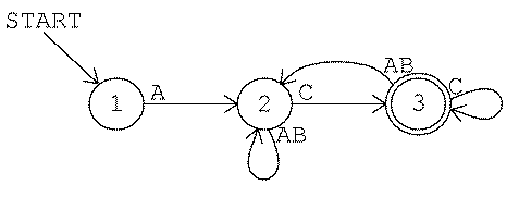
This machine is similar to the nondeterministic version. It has the same number of states and some of the connections are identical. State 3 is more complicated, though. Also, in this machine, it is no longer the case that each state of the machine corresponds exactly to one of three parts of the input string. Specifically, when the machine is in state 3 the string may or may not be finished.
The game program uses finite-state machines to represent the rules
by which it accepts or rejects strings. (The machines must be deterministic
for the program to work.) Logo programs can't read circles and arrows,
so a machine is represented as a list. What information is actually
contained in an FSM diagram? The diagram shows that there are a certain
number of states (the circles), that there are certain transitions from one
state to another (the arrows), that one particular state is the start state
(the start arrow), and that certain states are accepting ones (the double
circles). As in any programming project, I could have chosen many different
ways to represent that information in the program.
In the particular representation I chose, the list form of a machine has three members. The first member is the number of the start state. The second member is a list of arrows; each arrow is itself a list, as I'll explain in a moment. The third member of a machine list is a list of the accepting states of the machine. For example, here is the machine for game 3 again, in both forms:

[1 [[1 A 2] [2 B 3] [3 ABC 3]] [3]]
The number 1 is the start state; the list [3] is the
list of accepting states. (This machine happens to have only one accepting
state.) Everything else is the list of arrows. Each arrow is also a list
with three members: the initial state (the tail of the arrow), the input
letter or letters, and the final state (the head of the arrow). The first arrow in
this machine is
[1 A 2]
This is the arrow from state 1 to state 2 associated with
the input A.
The list [3 ABC 3] in this machine represents three arrows, using
the same shorthand as in the circle-and-arrow diagrams. I could equally
well have represented these arrows separately:
[1 [[1 A 2] [2 B 3] [3 A 3] [3 B 3] [3 C 3]] [3]]
As in the circle-and-arrow diagrams, I haven't explicitly represented the
transitions to the reject state in these lists. The program is
written so that if it doesn't find a transition for the current state and
input in the list of transitions, it goes into state number −1, its
representation for the reject state.
Here are some more machine lists:
Game 2:  [1 [[1 ABC 2] [2 ABC 1]] [1]]
Game 7:  [1 [[1 AB 1] [1 C 2] [2 C 1]] [1]]
Game 9:  [1 [[1 AB 1] [1 C 2] [2 A 3] [2 B 1] [3 A 1]] [1]]
At this point you should stop and play with the program. Make up
your own rules. The procedure fsm takes a machine list as input
and accepts strings based on that machine. (Game uses fsm
with particular
machines as inputs.) Try out your new rules to make sure you've designed
the machines correctly. Then get a friend to play with your rules.
If both of you are reading this book together you can have a competition.
(It's easy to design rules that are impossible to guess because there
are too many details. If you have a competition you should limit
yourselves to three states per machine.)
You might be interested in reading through the
fsm program, which
simulates a finite-state machine when given the machine's description
as its input. It's a pretty simple program. If you think of a machine's
state diagram as a kind of "wiring diagram" that might be used
in building a real version of that particular machine, this Logo program
is a kind of universal finite-state machine implementation.
It may seem to you that accepting or rejecting strings isn't much like what you usually do with computers. You may wonder how this mathematical model is related to real computer programming. There are two answers to this question. One is that it's possible to design finite-state machines that have more versatile outputs than simply yes or no. I'll give an example shortly. But the other answer is that there are real situations in which accepting or rejecting a string of symbols does come up in practical computation.
One example is in the implementation of programming languages. When you say that
print 2+2
is a legal Logo instruction but
print 2+
is illegal, you're doing a more complicated version of what a finite-state acceptor does.
The search command in a good text editor uses finite-state machines. Most text editors have a command that allows you to look through a file for a particular string of characters. Fancier editors allow searching not just for one particular string, but for any string that follows a rule the user can provide. The editor finds a string that matches the rule using a finite-state machine. Of course, people who use editors don't have to specify their search rules in the form of a finite-state machine! The editing program accepts search rules in a simpler form and translates them into FSM form. Here is an example, the notation used by ed, a standard editor in the Unix operating system.
A string like
spaghetti
just matches an identical string in the file you're editing. A slightly more interesting case is
[Ss]paghetti
which matches either "Spaghetti" or "spaghetti" (with a capital or lower case "s"). The square brackets indicate that any of the letters inside the brackets will be accepted. In the expression
[Ss]paghet*i
the asterisk matches any number (including zero) of the
letter before it (in this case, the letter t). This example
would match any of these:
Spaghei
Spaghettttti
spaghetti
spagheti
You might use this in a search command if you're a bad speller! The bracket and asterisk can be combined;
C[AD]*R
will match any of
CAR
CDR
CADDR
CR
Or you could use
M[is]*p*i
to match the name of a famous river.
Some of the rules from the game I presented earlier can be represented as
ed search strings according to these rules. In the first game the
machine accepted any string made up of As and Bs. The
corresponding ed expression is
[AB]*
The third game called for strings beginning with the sequence
AB, followed by whatever you like. This can be represented as
AB[ABC]*
Game 10, which I'm sure you didn't solve, accepts any string that
includes the sequence ABCBA within it. In ed terms, that's
[ABC]*ABCBA[ABC]*
I haven't given you a complete description of the ed search rules. I included this much only because I want you to see how a "real" program uses the idea of finite-state machines. But in the remaining part of this chapter I want to use a different notation based on Logo words and lists.
The notation I'm about to describe allows an acceptance rule, like the rules
in the game program or the rules for ed searches, to be
represented in Logo. The representation of such a rule is called a
regular expression. I'm going to tell you some rules for what a regular
expression can look like. Don't be confused: Any particular regular
expression is a rule that accepts strings of letters. I'm giving you rules
that accept regular expressions--rules about rules. As a rough analogy,
"one player is X and the other is O" is a rule about the
specific game Tic Tac Toe; "each player should have a fair chance to win"
is a rule about what kinds of game rules are acceptable.
Alphabet rule. Any symbol in a machine's
alphabet is a regular expression. We represent the symbol as a one-letter
Logo word. In our guessing game the alphabet contains three symbols:
A, B, and C. So
B
is a regular expression.
Concatenation rule. A list whose members are regular expressions
represents those expressions one after another. For example, since A
is a regular expression and B is a regular expression,
[A B]
is a regular expression representing the string AB. (Notice
that the Logo word AB does not represent that string; the
alphabet rule requires that each letter be represented as a separate word.)
Alternatives rule. A list whose first member is the word or and
whose remaining members are regular expressions represents any string that
matches any of those expressions. For example,
[OR [A A] B]
matches either the sequence AA or the single symbol B.
As a convenience, a Logo word containing more than one letter (other
than the word or) is taken as an abbreviation for the oring
of the individual letters. For example, ABC is equivalent to
[OR A B C].
Repetition rule. A list containing exactly two members, in which the
first is the asterisk (*) symbol and the second is a regular
expression, represents a string containing any number (including zero) of
substrings that match the regular expression. So
[* [OR [A A] B]]
matches any of these:
B
|
BB
|
BAAB
|
AAAAAA
|
AABAA
|
| (the empty string) |
AABBBBBAA
|
The number of consecutive As must be even for a string of
As and Bs to match this expression.
These four rules constitute the definition of a regular expression. It's a recursive definition. Just as the effect of a recursive Logo procedure is defined in terms of a simpler case of the same procedure, a complex regular expression is defined in terms of simpler ones.
Here are the ten game rules from the beginning of this chapter in the form of regular expressions:
| 1. | [* AB]
|
|---|---|
| 2. | [* [ABC ABC]]
|
| 3. | [A B [* ABC]]
|
| 4. | [* [OR [A A] [B B] [C C]]]
|
| 5. | [* [ABC B]]
|
| 6. | [A [* ABC] C]
|
| 7. | [* [OR A B [C C]]]
|
| 8. | [[* BC] [* [A [* BC] A [* BC]]]]
|
| 9. | [[* AB] [* [C [OR B [A A]]] [* AB]]]
|
| 10. | [[* ABC] A B C B A [* ABC]]
|
You should go through these examples carefully, making sure you understand how the regular expression represents the same idea as the English description or the machine diagram you saw earlier.
You may be thinking that any rule for accepting or rejecting strings of symbols can be represented as a regular expression. But that's not so. For example, consider the rules for recognizing ordinary arithmetic expressions:
| accepted | rejected |
|---|---|
2+3 | 23+
|
2*(3+4) | 2*)3+4(
|
-5 | /6
|
Think for a moment just about the matter of balancing parentheses. Sometimes you have parentheses within parentheses, as in
((3+4)/(5+6))
How would you represent this part of the arithmetic expression rule in the form of a regular expression? You can't just say something like
[[* (] something-or-other [* )]]
to mean "any number of open parentheses, something, then any number of close parentheses." That would allow strings like
(((7)))))
But this string should be rejected because it has too many close parentheses. You're not allowed to use a close parenthesis unless you've already used a matching open parenthesis. You can have any number of nested parentheses you want as long as they're balanced.
It is possible to invent other kinds of formal notation, more powerful than
regular expressions, that will allow us to give the rules for well-formed
arithmetic expressions. In this section I'll introduce briefly a formal
notation called production rules that's powerful enough to describe
arithmetic expressions. For now, in this chapter, I don't want to discuss
production rules in great detail; my only reason for introducing them at
this point is to give you a sense of how regular expressions fit into a
larger universe of possible formal systems. In the following sections I'll
have more to say about regular expressions and finite-state machines. But
we'll return to production rules in Chapters 5 and 6, in which we'll need
formal notations with which to discuss more interesting languages than the
A-B-C language of this chapter. (In Chapter 5 we'll be
talking about Pascal; in Chapter 6 we'll take on English.)
The key ingredient that's missing from regular expression notation is a way to name a kind of sub-expression so that the name can be used in defining more complex expressions. In particular, a sub-expression name can be used in its own definition to allow a recursive definition of the rule.
A production rule has the form
name : expansion
Each rule is a definition of the name on the left in terms of smaller units, analogous to the definition of a Logo procedure in terms of subprocedures. The expansion part of the rule is a string of symbols including both members of the "alphabet" of the system (like the alphabet that underlies a regular expression language) and names defined by production rules.
As an example, here is a set of production rules that defines the language of arithmetic expressions. These rules take into account the "order of operations" for arithmetic that you learned in elementary school: multiplication before addition. An expression like
2/3+1/6
is ordinarily interpreted as the sum of two terms, namely two thirds and one sixth. An expression can be a single term, a sum of terms, or a difference of terms. Here's how that idea is expressed in a set of production rules; I'll discuss the notation in more detail in a moment.

The vertical bars separate alternatives. The first rule, the one
that defines expr, contains three alternatives. First, an expression
can be just a single term. Second, an expression can be a smaller
expression plus a term. Third, an expression can be a smaller expression
minus a term. The symbols inside boxes are the members of the alphabet of
the arithmetic expression language. (I've put them in boxes to make it
easier not to confuse them with the punctuation characters--the colons and
vertical bars--that are part of the production rule notation itself.)
Do you see how parentheses fit in? If a string like 4+5 is an
expression, then (4+5) is a factor, so 3*(4+5) is a term,
and so on. Since a factor is a kind of term, and a term is a kind of
expression, the factor (4+5) can be considered an expression, and
so it too can be put inside parentheses. So ((4+5)) is also
acceptable as a factor.
I've hinted at something that I haven't actually made explicit: Regular expressions are equivalent to finite-state machines. In other words, if you can express a rule as a regular expression, you can design a finite-state machine that carries out the rule. If you can't write a regular expression for the rule, you can't design a finite-state machine either.
You may be thinking, "so what?" I've introduced two different formal notations, finite-state machines and regular expressions, and now I'm telling you that the two are equivalent. So why didn't I just pick one in the first place and forget about the other? I have a general answer and a specific answer to these questions.
The general answer is that comparing different formal systems is what automata theory is all about. By the end of this book you'll have been introduced to half a dozen or so different formal systems. Some are more powerful than others. The bare assertion that one formal system is equivalent to another, or more powerful than another, isn't very interesting; but if we can understand the reasons behind those assertions then we may be able to put the knowledge to work in practical situations. At the very end of this book, in Chapter 6, we'll talk about a particular formal system that's often used in artificial intelligence programs to recognize English sentences. By then you should know enough about formal systems to be able to understand why that particular one is a good choice.
The specific answer is that finite-state machines and regular expressions are different from each other in an interesting way. A finite-state machine is an algorithm, a sequence of steps, or a procedure that can be followed to test whether some string matches a given rule. It says, "start here, then if this happens do this, then..." just like a procedure in Logo or most other programming languages. (But we've seen that a finite-state machine is like a procedure written in a restricted programming language that isn't as flexible as Logo.) A regular expression, though, is not a sequence of steps. It's more like a description of the result that we want, leaving open the precise recipe for how to get there. People often pose problems in a similar way. They call the plumber and say, "the drain in my bathtub is backing up." Part of the plumber's expertise is to be able to translate that declarative problem statement into a procedural form, a sequence of steps needed to clear up the problem. An early stumbling block in artificial intelligence research was the seeming gulf between the procedural knowledge embodied in a computer program and the declarative knowledge needed for human-like behavior. Recently people have invented declarative programming languages (the best known is Prolog, but any commercial spreadsheet program is also in this category) that allow the user to state a problem in declarative form. The programming language interpreter then automatically translates this problem statement into a sequence of steps for the computer to perform.
Writing a Prolog interpreter raises many issues beyond the scope of this
book. But we can take a smaller step in the realm of translation from
a declarative notation to a procedural one. I've written a Logo program,
listed at the end of the chapter, that translates from a regular
expression to an equivalent finite-state machine. Its top-level procedure,
machine, takes a regular expression as input and outputs a machine
list in the format I showed earlier.
The general claim that regular expressions are equivalent in power to finite-state machines is called Kleene's Theorem, named after the mathematician Stephen C. Kleene, its discoverer. You can find a proof of this theorem in any textbook on automata theory. I'm not going to give a proof here, but I'll indicate how the translation is done in my program. The same kinds of ideas are used in the proof.
Remember that there are four parts to the definition of a regular expression.
The alphabet rule provides the fundamental building blocks; the
concatenation, alternatives, and repetition rules build large regular
expressions recursively out of smaller ones. The translation process
follows the same pattern: We start with a procedure to build a trivial
two-state machine that only accepts a single letter, then we add three
rules for combining smaller machines into a large machine. In the following
paragraphs I'll show how each rule is reflected in the
machine program.
This construction process often produces machines with more states than
necessary. The machine program eliminates redundant states as its
final step.
The alphabet rule says that any member of the machine's alphabet is
a regular expression. In the program, a symbol can be any one-letter word other
than *. The symbol X is translated into the machine
[1 [[1 X 2]] [2]]
(You'll see that the program works by combining little machines
into bigger ones. Every time the program has to invent a new machine
state it uses the next free number. So the state numbers might not
be 1 and 2 in a real example.) The procedure
ndletter handles this
rule.
Next comes the concatenation rule. The regular expression
[A B]
matches a string with two parts; the
first substring matches the A and the second matches the
B. In this simple example each "substring" matches only a single
letter. In a more complicated concatenation like
[[OR A C] [* B]]
there are different choices for each substring. For example, that regular expression is matched by the string
CBBB
in which the letter C matches the first part of the
expression and the substring BBB matches the second part.
To translate a regular expression of this kind (a concatenation) into a
finite-state machine, we begin by recursively translating the subexpressions
into smaller machines. Then we have to "splice" the two machines together.
Procedure ndconcat does this splicing.
We'll begin with the simplest possible example. Suppose we want to translate the regular expression
[A B]
We have already translated the two symbols A and B into
machines:

The combined machine must start at the start state of the first component machine, state 1. The combined machine should be in an accepting state when both component machines have been satisfied; in other words, the accepting states of the combined machine should be those of the second component machine. In this case that means only state 4.
To splice the component machines together we must add transitions (arrows)
between them. Specifically, whenever the first component machine gets into
an accepting state, the combined machine should follow the same transitions
that apply to the start state of the second component machine. In this
case, when the combined machine gets into state 2 (the accepting state of
the first component machine) it should follow the same transitions that
apply to state 3 (the start state of the second machine). There is only one
such transition, a B arrow into state 4. That means we must add the
arrow
[2 B 4]
to the combined machine.

State 3, although it is still in the machine, is now useless. There is no way for the machine to get into state 3. Later in the translation process another procedure removes such "orphaned" states from the machine.
As a slightly more complicated example, consider the translation of the regular expression
[[OR A C] [* B]]
We start by supposing that we've already translated the two subexpressions separately:
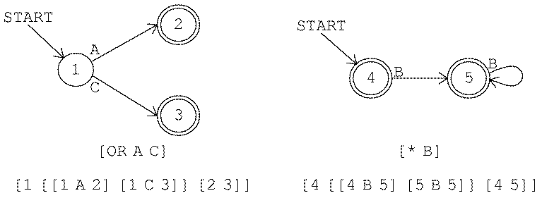
(We haven't yet discussed the alternatives rule or the repetition rule, so I haven't yet explained how these subexpressions are translated. For now, please just take on faith that this picture is correct. We'll get to those other rules shortly.)
The start state of the combined machine is the start state of the first component, state 1. At every accepting state of the first machine we must duplicate the transitions from the start state of the second machine. In this example the start state of the second machine has only the transition
[4 B 5]
but there are two accepting states in the first machine, so we must add two new arrows:
[2 B 5] [3 B 5]
A final detail is that in this example the start state of the second component machine, state 4, is an accepting state. That means that the second substring can be empty. Therefore the accepting states of the first component machine should also be accepting states of the combined machine. Here is the result:
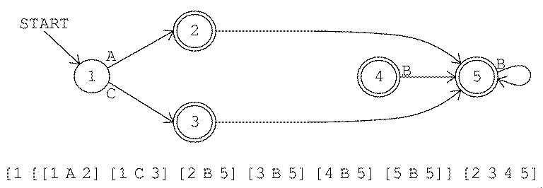
Again, state 4 is now an "orphan" and will be eliminated later in the program.
The alternatives rule combines two machines in parallel, so to speak,
rather than in series. It works by inventing a new state
that becomes the start state of the combined machine. Arrows leaving
from the new state duplicate the arrows from the start states of the
component machines. Procedure ndor handles this rule.
As an example, here is the translation process for
[OR A B]
(or its abbreviation AB). We start with two separate machines:
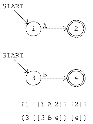
We combine them by inventing a new state 5:
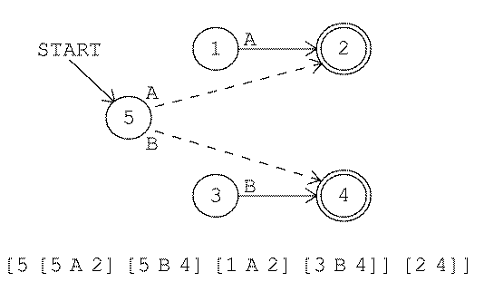
I haven't explained all the details of the construction process. For example, should the new state, state 5, be an accepting state? In this example it shouldn't be. See if you can think of a case where it might be; then read the program listing to see the exact algorithm that makes this decision. Again, this construction process may leave unused states for later cleanup.
A much more serious problem is that an or construction is likely to
produce a nondeterministic machine. For example, here is the machine
for
[OR [A B] [A C]]
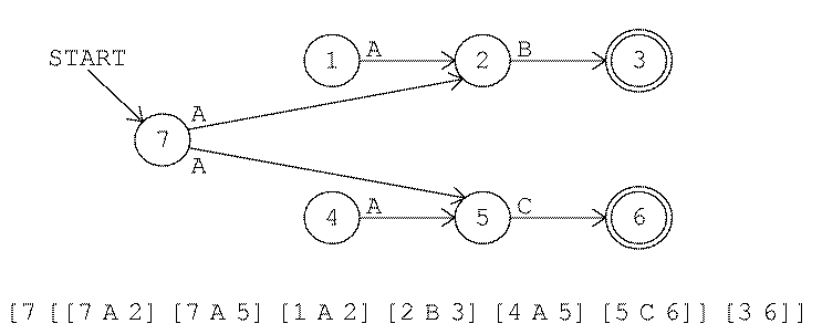
Like the unused states, the problem of nondeterminism is
left for the end of the program, when procedure determine translates
the nondeterministic machine into a deterministic one.
(The concatenation rule can also make nondeterministic machines, although
it's not as likely.)
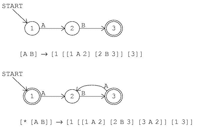
The final case to be considered is the repetition rule. This rule
acts on only one smaller machine, not two machines as in the previous
two cases. The rule doesn't require any new states. It has two effects.
One is to add the start state to the list of accepting states. The
second is to add arrows from the (old) accepting states that mimic
the arrows from the start state. (This is exactly like the splicing
of two machines in the concatenation rule, but in this case we concatenate
a single machine with itself!) Procedure ndmany
makes this transformation.
It, too, can result in a nondeterministic machine.
Here is an example of the rule:
These four rules are combined by nondet,
a procedure whose input is
a regular expression and whose output is a (possibly nondeterministic) machine.
to nondet :regexp
if and (wordp :regexp) (equalp count :regexp 1) [output ndletter :regexp]
if wordp :regexp [output ndor reduce "sentence :regexp]
if equalp first :regexp "or [output ndor butfirst :regexp]
if equalp first :regexp "* [output ndmany last :regexp]
output ndconcat :regexp
end
The top-level procedure machine
does a little initialization
and then does its work with the instruction
output optimize determine nondet :regexp
That is, first it creates what may be a nondeterministic machine, then if necessary it translates that into a deterministic one (eliminating orphan states in the process), then it gets rid of any redundant states that may have been created.
In the first volume of this series we explored the techniques of depth-first and breadth-first tree traversal. Given a tree structure, these algorithms allow us to "visit" every node of the tree once.
A finite state machine can be viewed as a structure almost like a tree. The machine's start state corresponds to the root node; the states that can be reached by an arrow from a given state are the children of that state. But there is one important difference between trees and machines: In a tree, every node (except for the root node) has exactly one parent. The tree search algorithms depend on that fact to ensure that each node is visited only once. In a machine, arrows from several different states can lead to the same state, so a state may have several "parents." The technical name for an arbitrary collection of nodes with connections among them is a graph. If the connections are one-way, as in the finite state machine diagrams, it's called a directed graph.
Searching a graph is just like searching a tree, except that we have to
keep track of which nodes we've already visited, to avoid examining the
same node twice. Procedure determine
creates a list named states, initially
empty, into which each state number is added as the
program examines that state. The depth first traversal of the machine
is carried out by procedure nd.traverse;
although this procedure looks different from the
depth.first
procedure in Volume 1, it
uses the same basic algorithm. Given a state as input, it processes
that state and invokes itself recursively for all of the children of
that state--the states reachable by arrows from the input state. Unlike
depth.first, though, nd.traverse is an operation. It
outputs a new list of moves (arrows) for the deterministic version of
the machine.
What does it mean to process a state? Nd.traverse first checks
whether this state has already been processed; if so, it outputs an empty
list, because this state will contribute no new moves to the machine.
Otherwise, it remembers this state number as having been processed, finds
all the moves starting from this state, and calls
check.nd to look for
nondeterminism. Check.nd takes the first available arrow whose tail
is at the state we're processing, and looks for all arrows with the same
tail and with the same letter.*
The local variable heads will contain a list of all the state numbers
reachable by these arrows. (The state numbers are sorted into increasing
order, and duplicates eliminated. If the machine has two completely
identical arrows, that doesn't result in nondeterminism.)
*By the way,
nondet always
creates arrows with only a single letter; if two or more letters lead from
the same state to the same state, a separate arrow is created for each of
them. This makes for a longer machine list, but makes steps like this
one--looking for two arrows with the same letter--easier. Once the
deterministic machine has been created, procedure optimize will combine
such arrows into the abbreviated form with
more than one letter per arrow.
There are
three cases for what check.nd must do. First, if there is
only one state number in :heads, then there is no nondeterminism for
this letter, and check.nd includes the arrow from the original
machine as part of the deterministic machine. Second, if there is more
than one state number, check.nd looks to see if we've already seen
the same combination of result states. If so, then we've already created
a new state equivalent to that combination of old states, and check.nd
creates a new arrow pointing to that existing new state. Finally, the third
case is that this combination of states is one we haven't seen before. In
that case, check.nd must create a new state, with arrows duplicating
those from all of the original states.
In other words, if there are arrows
[[3 B 4] [3 B 7]]
then check.nd will invent a new state that is an "alias"
for "four-and-seven." If the same machine also contains arrows
[[8 C 4] [8 C 7]]
then check.nd will use the same alias state for this
pair, not inventing a new one. The new
state is given arrows matching those of all its component states (4
and 7 in this example). The new state might itself contain a nondeterministic
branch, but that's okay because the new state will eventually be processed
as we continue to traverse the machine graph.
You might think that this process could go on forever: that each new
state check.nd invents will turn out to include nondeterminism, which
will require yet another new state to resolve. Fortunately, that
doesn't happen; the process does always end eventually. (In the next
chapter we'll see what the limit is on the number of necessary states
for the deterministic machine.)
Because determine uses a graph traversal algorithm to examine
the original machine's states, it will never find "orphan" states
that can't be reached by arrows from some other state. That's why
the process of making the machine deterministic also eliminates orphan
states, with no extra effort.
The machines produced by determine are runnable, but often ugly;
they contain many more states than necessary. Procedure
optimize
eliminates many redundancies and also combines arrows with the same
head and tail but with different letters.
First it goes through the machine's arrow list,
creating a list for each state representing the exits from that state:
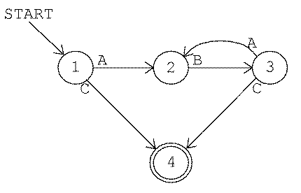
   [[* [A B]] C]
State 1: [[A 2] [C 4]]
State 2: [[B 3]]
State 3: [[A 2] [C 4]]
State 4: []
In this machine, states 1 and 3 have the same exit list. (In these lists, each arrow is represented with only two members; the arrow's tail is not included. That's because states 1 and 3 would not have identical lists if the tails were included. State 1's list would be
[[1 A 2] [1 C 4]]
and state 3's list would have arrows starting with 3. In the program, the two-member form of an arrow is called a stub.)
The program must be careful about the order in which it puts stubs in each state's list, so it doesn't end up with
[[C 4] [A 2]]
for one of the states. That's why stub.add
takes trouble
to insert each stub in a well-defined position, rather than just adding
each new stub at the beginning or end of the list. It's also in
stub.add that arrows connecting the same two states but with different
letters are combined into a single arrow.
Since states 1 and 3 also agree in their acceptingness (namely they aren't
accepting states), they can be combined into one state.
Optimize.state can replace every reference to state 3 with a reference to
state 1.
I promised earlier to show you a use for finite-state machines other than accepting or rejecting strings. In this section I'll fulfill that promise by designing a machine to add two numbers. We'll represent the numbers in binary notation, in which each digit represents a power of 2 instead of a power of 10.
If you've come across binary numbers before, you can skip this paragraph. Just as the ordinary notation for numbers is based on the ten digits 0 to 9, binary notation is based on two digits, 0 and 1. In ordinary ("decimal") notation, the amount that each digit contributes to the total depends on where it is in the number. For example, in the number 247, the digit 2 contributes two hundred, not just two, because it's in the third position counting from the right. Each digit's contribution is the value of the digit itself multiplied by a power of ten:
(102 is 100; 101 is 10; 100 is just 1.) In binary, the contribution of each digit is multiplied by a power of two, so the binary number 10101 represents
which is 16+4+1 (24+22+20) or 21. Computers use binary notation because it's easy to build electrical circuits in which each wire is either on or off. In Chapter 2 we'll talk about an example. Right now I want to show something different--not an actual electronic machine but an abstract machine based on the ideas we've been using in this chapter.
The machine will add two binary numbers, one digit position at a time, just the way you add multi-digit numbers yourself. When you see a problem like
| 376 |
| +572 |
you start at the right and say, "6 plus 2 is 8; 7 plus 7 is 14, which is 4 carry 1; 1 plus 3 plus 5 is 9." The finite-state adder works the same way except that the digits are always 0 or 1.
The machine will add any numbers, but to explain how it works I want to consider a specific example. Let's say we want to add 52 and 21. (By the way, I didn't pick these numbers because they name card games, but because the pattern of digits in their binary forms is convenient for the explanation I want to give.) 52 in binary is 110100 (32+16+4) and 21 is 10101 (16+4+1). I'm going to write these one above the other, with a couple of extra zeros on the left to leave room for a possible carry:
          0 0 1 1 0 1 0 0
          0 0 0 1 0 1 0 1
Remember how a finite-state machine works: At a given moment it's
in some state, then it reads some input symbol and goes to
another state. In this problem, since we have two numbers to add, the most
natural way to think about it would be to give the machine two inputs
at a time. This idea doesn't quite fit in with the formal definition of a
finite-state machine, but we can let the machine's "alphabet" consist of
pairs of digits, so something like 01 would be a single input.
(By the way, the word bit is commonly used as an abbreviation for
"binary digit.") Just as you added vertical pairs of digits (first 6 and 2,
then 7 and 7, and so on) in the earlier example, we'll use vertical pairs of
bits as the inputs to the finite-state adder, starting from the right end.
So the first input will be 01, then 00, then 11, then 00, then 11 again,
then 10, and then 00 twice. From now on, in this section, when you see
something like 10 you should remember that it is a single input to
the finite-state machine, a single symbol, not two in a row.
(In the diagram below, an arrow labeled 01/10 represents two
arrows, one for the input 01 and one for the input 10. These
two arrows will always go to the same state because 0+1=1+0.)
We need to make one change in the notation used in machine diagrams. We no longer want to mark each state as accepting (double circle) or rejecting (single circle). Instead, each state produces an output that can be any arbitrary symbol. In this machine the outputs will be 0 or 1, representing the binary digits of the sum. Inside each state circle, instead of just a state number you'll see something like "3/1"; this means that it's state number 3 and that the output from that state is 1.
Here is the machine:
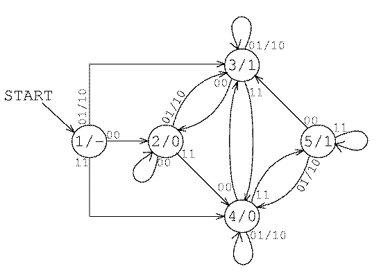
State 1, the start state, has no output. When the machine is in start state it hasn't seen any digits of the addends yet, so it can't compute a digit of the sum. States 2 and 4 output a zero digit, while states 3 and 5 output a one. (Like the inputs, the number that the machine outputs is presented with its rightmost bit first. The machine works this way for the same reason that you add numbers from right to left: That's the direction in which a "carry" digit moves from one column to another.)
Why are there two zero-output states and two one-output states? The reason is that the machine is in state 4 or 5 when there is a carry into the next digit of the sum.
Let's trace through my example. We start in state 1. The first input symbol is 01, representing a 0 in the rightmost (binary) digit of 52 and a 1 in the rightmost digit of 21. The machine enters state 3 and outputs a 1.
The next input is 00 because both numbers have zero as the second digit. The machine enters state 2 and outputs 0.
The next input is 11. The machine enters state 4 and outputs 0. Being in state 4 means that there is a carry from this position into the next.
You can finish the example yourself. The sum should be 01001001, or 73.
Earlier we saw that you can't write a regular expression for a rule that requires balanced parentheses. Since regular expressions are equivalent to finite-state machines, you won't be surprised to learn that finite-state machines can't count.
Actually, they can count up to a point; it's just that each finite-state machine can only count up to a fixed limit. For example, here is a finite-state machine that accepts strings of balanced parentheses up to four deep:

This machine will accept strings like these:
          ()        (())      ()()
          (()())    (((())))  (((())))(())
There is no limit to the length of the string this machine can handle. For example, it will accept this:
()()()()()()()()()()()()()()
But there can be no more than four parentheses open at once; the machine will reject
((((()))))
Even this limited counting ability of finite-state machines is of great practical value. Real computers, after all, are finite-state machines. Any real computer has a finite amount of memory, and this memory can be in a finite number of states. But the number is quite huge. If a real computer includes a parenthesis-counting program that is limited to, say, 20,000 levels of parentheses, nobody will ever notice that the limit isn't infinite.
(The number of states in a real computer may be even larger than you're thinking. Each bit of computer memory isn't a state. Instead, if a computer has n bits of memory it has 2n states! For example, a computer with three bits of memory can use those bits to represent eight states:
0 0 0
0 0 1
0 1 0
0 1 1
1 0 0
1 0 1
1 1 0
1 1 1
The number of possible states in a typical large computer is greater than the number of atoms in the galaxy.)
In a moment I'm going to talk about a theoretical model of a machine with infinite memory. You might wonder why it pays to study such machines, since any real machine has to be limited in memory. The answer has to do with my example about the 20,000 levels of parentheses. It is theoretically possible to write a regular expression for such strings. To show you how it's done, here is a regular expression for up to three levels:

(I've drawn boxes around the actual alphabet-rule symbols just to make it a little easier for you to distinguish between the parentheses, which are symbols in the input strings, and the brackets, which are part of the glue that holds a regular expression together.)
There is no theoretical problem about extending this regular expression to allow up to 20,000 parentheses. But a machine based on this technique would be very large and complicated. Instead, it makes more sense to pretend that the computer has an infinite amount of memory available and use a formal system (like the production rules I mentioned briefly) that depends on an infinite memory. Such a formal system leads to a shorter, more elegant expression of the balanced parentheses rule. In practice, we can provide enough memory for any of the strings our program will actually meet.
One way we might explore infinite machines is to imagine that they're represented by state diagrams, like those of finite-state machines, but with an infinite number of states. For example, here is a picture of an infinite-capacity parenthesis counter:

The trouble with this idea is that it's hard to model precisely what's meant by that row of dots on the right. There's no way we can have a complete formal description of an infinitely complex machine.
Instead, consider what you do when you have to solve a problem too complex to fit in your own memory. You don't build yourself a bigger brain; you get a pencil and some paper. That is, you use external storage. You can imagine that your brain is a finite-state machine but that it has access to an infinite supply of paper.
Of course, this division of a problem's necessary information into a finite internal state and an infinite external memory also models actual computers in an obvious way. The internal state in the model represents the internal memory of the computer, while the external memory in the model represents such storage devices as disks and tapes. To solve a bigger problem you don't have to buy a bigger computer; you just have to switch floppy disks occasionally.
You might think that the mathematical model I'm talking about was based on the analogy with real computers and that my story about the finite-state brain is just a coincidence. But in fact this model was invented by Alan M. Turing in 1936, before there were any computers! It was human problem-solving that Turing wanted to model with a machine.
What is a Turing machine? Start by imagining a finite-state machine with different possible outputs, like the adder we saw earlier. Attached to this machine is a tape of limitless length. Symbols from some alphabet, like the machine's input and output symbols, can be written on the tape. There is a reading and writing mechanism, like the heads of a magnetic tape recorder, that can travel along the tape.
Just as each state of the machine can have an output associated with it, each state can also take action to affect the tape: It can move the head by one symbol in either direction and it can change the symbol at the head's current position.
In fact, we simplify the formal description of the machine by using the tape as the input/output device as well as the storage device. That is, we can start with some sequence of symbols already written on the tape. That sequence serves as the input to the machine; state transitions are based on the symbol under the tape head, not a symbol from some other source. Likewise, the output from a state (if any) is written on the tape.
Somewhat analogous to the concept of an accepting state in our earlier examples, a Turing machine can have halting states. When the machine enters a halting state it stops its operation. There are no more state transitions. The output from the machine is whatever sequence of symbols it leaves written on the tape.
Turing invented his abstract machine because he was trying to formalize the idea of an effective procedure: What does it mean to specify a technique for solving some problem well enough that we can be sure it will really work? As an analogy, think about directions for driving from here to somewhere. Someone can hand you a piece of paper with a list of instructions like "When you get to the gas station on the left, turn right." But sometimes you get directions that weren't careful enough. There may be a sharp right turn and a mild right turn available near the gas station. There may be a fork in the road before you even get to the gas station.
Turing's idea is that any problem for which there is any effective procedure can be modeled by a Turing machine. The phrase "any effective procedure" is taken to include the workings of the human mind. If Turing is right, any problem that a person can solve can be programmed for a computer.
This claim isn't something that can be proved or disproved mathematically because there is no prior formal definition of "effective procedure" to which Turing machines can be compared. Also, it may be that the idea of a procedure somehow doesn't cover all the different kinds of thinking that people do. Maybe it's true, for example, that computers are potentially as powerful as people at solving problems, but "solving problems" might not turn out to be an appropriate description of what's going on when we feel emotions. If that turned out to be true, we should expect a computer to become the world's chess champion someday, but we shouldn't expect one to become the world's champion poet.
But this possible conclusion has been attacked from both sides. Some people think that emotions really are a matter of computable procedures. Kenneth Colby's program called Parry attempts to model the behavior of a paranoid human being by manipulating variables for emotions like anger and fear. On the other hand, some people think that even chess doesn't fall within the realm of things that people do by carrying out effective procedures in Turing's sense. A chess master, these people say, doesn't analyze the chess board in a step-by-step fashion like a computer. He looks at the board as a single, whole entity, and the important features just spring to mind by some process that is still rather mysterious.
What is known is that several other mathematical models of effective procedures have been shown to be equivalent to Turing machines, in the same sense in which regular expressions are equivalent to finite-state machines. For example, all of the popular programming languages are Turing-equivalent. There's no such thing as a computation that can be done in Logo but not in Pascal, or vice versa. (Of course, one language may be more convenient than another for a given problem.)
I'm not going to get into specific examples of Turing machine programming here. That would take too much space for a single chapter; if you're interested you should pursue the topic in a book on automata theory. But I want to give one example of the theoretical value of Turing machines.
You've undoubtedly had the experience of writing a Logo program with a bug
that causes an "infinite loop"--you run the program and it just sits there
forever, when instead it's supposed to compute and print some results.
That's a frustrating kind of bug because you're never quite sure if the
program is really broken or if it's just very slow. Maybe if you waited
another minute it would come up with the answer. Wouldn't it be great if,
when you started the program running, Logo could print an error message like
This program has an infinite loop, just as it does for other errors?
It turns out that infinite loops can't, in general, be detected automatically. Certainly some infinite loops are very easy to spot, and we can write programs that catch certain categories of infinite loop. But we can't write a program that's guaranteed to catch infinite loops in programs, in Logo or any other Turing-equivalent language. The fact that it's impossible is called the halting theorem.
It's a little tricky understanding just what the halting theorem says because it involves Turing machines that manipulate Turing machines as data, which is a kind of self-reference akin to recursion. Self-reference is always hard to talk about and can lead to paradoxes like the classic "This statement is false." (Is the sentence in quotes true or false? If it's true, then it must be false, because it says so. But if it's false, and it says it's false, it must really be true!) So let's proceed carefully.
The data recorded on a Turing machine's tape is a string of symbols. Generally we choose the symbols to represent something meaningful; for example, a string of digits can represent a number. Earlier in this chapter we used strings of symbols like
[1 [[1 A 2] [2 B 3] [3 A 2]] [1 3]]
to represent a finite-state machine. There's no reason we
couldn't put that string of symbols on the tape of a Turing machine
as its input. For example, we could build a Turing machine that would work
like my fsm program, simulating the finite-state machine that it found
written on its tape when it started.
Letting a Turing machine simulate a finite-state machine doesn't raise questions of self-reference. But a Turing machine, too, is a formal structure; it, too, can be represented as a string of symbols.
Because a representation of a Turing machine can be the input to another
Turing machine, we can design Turing machines that answer questions about
Turing machines. For example, we can write a universal Turing
machine, one that simulates any Turing machine the way fsm simulates
any finite-state machine.
A universal Turing machine (a Turing machine simulator) sort of half-solves the halting problem. Suppose we want to know whether a given machine will halt after it is started with a given input. (This is like asking whether a certain Logo procedure will terminate if it's invoked with a particular input.) We can use the universal Turing machine to simulate the one we're interested in. If the machine does halt, we'll find out about it. But if the machine in question doesn't halt, then the simulator won't halt either. We'll still have the problem we had in the first place--how can we be sure it won't finally halt if we give it another minute?
To solve the halting problem, what we need is a Turing machine that accepts a representation of any Turing machine as input, just like the universal Turing machine. But this one has to be guaranteed to halt, even if the input machine wouldn't halt. That's what the halting theorem says we can't do.
What makes it possible to raise the question of whether a Turing machine can
decide whether another Turing machine would halt for a given input tape is
the fact that one Turing machine's "program" can be represented as data
for another Turing machine. This is also true of Logo procedures. In
particular, the higher-order procedures like map and filter
manipulate other procedures by accepting their names as inputs.
We can, therefore, use Logo
procedures to illustrate the proof of the halting theorem.
We'll consider a Logo procedure with an input as analogous to a Turing machine with its input tape. We want to prove that there can't be a Logo procedure that could tell whether such a procedure stops for a given input. The technique we use is called proof by contradiction. In this technique we assume that there is such a procedure, then show that this assumption leads to a paradox.
So let's imagine that someone has written a Logo predicate haltp that
takes two inputs: the name of a procedure and an input value for that
procedure. Haltp will output true if the procedure it's testing
would eventually stop, given the specified input; haltp outputs
false if the procedure it's testing would get into an infinite loop, like a
recursive procedure without a stop rule. (In practice, if you think about
your own experience debugging programs, it's easy to tell if a procedure
doesn't have a stop rule at all, but not so easy to be sure that the stop
rule will always eventually be satisfied. Think about a Pig Latin program
given a word of all consonants as input. We want
to piglatin :word
if memberp first :word [a e i o u] [output word :word "ay]
output piglatin word bf :word first :word
end

? print haltp "piglatin "salami
true
? print haltp "piglatin "mxyzptlk
false
Remember that haltp itself must always stop, even
in the case where piglatin wouldn't stop.)
Now consider this Logo procedure:
to try :proc
if haltp :proc :proc [loop]
end

to loop
loop
end
Since haltp works, we're assuming, on any Logo
procedure with one input, it must work on try in particular.
What happens if we say
? try "try
Does this stop or loop? Suppose it stops. try begins its
work by evaluating the expression
haltp "try "try
Since we've said try will stop, given try as input,
haltp will output true. It follows, from the definition of
try, that try will invoke loop and will not stop.
Similarly, if we start with the assumption that try will loop, then
haltp must output false and so, from the definition of
try, you can see that try will stop. Whatever value
haltp outputs turns out to be incorrect.
It was the assumption that we could write an infallible haltp that led
us into this contradiction, so that assumption must be wrong. We can't write
a Logo procedure that will automatically detect infinite loops in our
programs. A similar proof could be made in any language in which one program
can manipulate another program as data--that is, in any Turing-equivalent
language.
| (back to Table of Contents) | BACK chapter thread NEXT |
;;; Finite State Machine Interpreter (FSM)

to game :which
fsm thing word "mach :which
end

to fsm :machine
cleartext
setcursor [0 3]
localmake "start startpart :machine
localmake "moves movepart :machine
localmake "accept acceptpart :machine
fsm1 :start
end

to fsm1 :here
ifelse memberp :here :accept [accept] [reject]
fsm1 (fsmnext :here readchar)
end

to fsmnext :here :input
blank
if memberp :input (list char 13 char 10) ~
   [print ifelse memberp :here :accept ["| ACCEPT|] ["| REJECT|]
    output :start]
type :input
catch "error [output last find [fsmtest :here :input ?] :moves]
output -1
end

to fsmtest :here :input :move
output and (equalp :here arrowtail :move) ~
           (memberp :input arrowtext :move)
end

;; Display machine state

to accept
display "accept
end

to reject
display "reject
end

to blank
display "|      |
end

to display :text
localmake "oldpos cursor
setcursor [15 1]
type :text
setcursor :oldpos
end

;; Data abstraction for machines

to startpart :machine
output first :machine
end

to movepart :machine
output first bf :machine
end

to acceptpart :machine
output last :machine
end

to make.machine :start :moves :accept
output (list :start :moves :accept)
end

;; Data abstraction for arrows

to arrowtail :arrow
output first :arrow
end

to arrowtext :arrow
output first butfirst :arrow
end

to arrowhead :arrow
output last :arrow
end

to make.arrow :tail :text :head
output (list :tail :text :head)
end

;; Machine descriptions for the guessing game

make "mach1 [1 [[1 AB 1]] [1]]
make "mach2 [1 [[1 ABC 2] [2 ABC 1]] [1]]
make "mach3 [1 [[1 A 2] [2 B 3] [3 ABC 3]] [3]]
make "mach4 [1 [[1 A 2] [1 B 3] [1 C 4] [2 A 1] [3 B 1] [4 C 1]] [1]]
make "mach5 [1 [[1 ABC 2] [2 B 1]] [1]]
make "mach6 [1 [[1 A 2] [2 AB 2] [2 C 3] [3 AB 2] [3 C 3]] [3]]
make "mach7 [1 [[1 AB 1] [1 C 2] [2 C 1]] [1]]
make "mach8 [1 [[1 A 2] [1 BC 1] [2 A 1] [2 BC 2]] [1]]
make "mach9 [1 [[1 AB 1] [1 C 2] [2 A 3] [2 B 1] [3 A 1]] [1]]
make "mach10 [1 [[1 A 2] [1 BC 1] [2 A 2] [2 B 3] [2 C 1]
                 [3 A 2] [3 B 1] [3 C 4] [4 A 2] [4 B 5] [4 C 1]
                 [5 A 6] [5 BC 1] [6 ABC 6]]
              [6]]


;;; Regular Expression to FSM Translation (MACHINE)

to machine :regexp
localmake "nextstate 0
output optimize determine nondet :regexp
end

;; First step: make a possibly nondeterministic machine

to nondet :regexp
if and (wordp :regexp) (equalp count :regexp 1) ~
   [output ndletter :regexp]
if wordp :regexp [output ndor reduce "sentence :regexp]
if equalp first :regexp "or [output ndor butfirst :regexp]
if equalp first :regexp "* [output ndmany last :regexp]
output ndconcat :regexp
end

;; Alphabet rule

to ndletter :letter
localmake "from newstate
localmake "to newstate
output (make.machine :from
                     (list (make.arrow :from :letter :to))
                     (list :to))
end

;; Concatenation rule

to ndconcat :exprs
output reduce "string (map "nondet :exprs)
end

to string :machine1 :machine2
output (make.machine (startpart :machine1)
                     (sentence (movepart :machine1)
                               (splice acceptpart :machine1 :machine2)
                               (movepart :machine2))
                     (stringa (acceptpart :machine1)
                              (startpart :machine2)
                              (acceptpart :machine2)))
end

to stringa :accept1 :start2 :accept2
if memberp :start2 :accept2 [output sentence :accept1 :accept2]
output :accept2
end

;; Alternatives rule

to ndor :exprs
localmake "newstart newstate
localmake "machines (map "nondet :exprs)
localmake "accepts map.se "acceptpart :machines
output (make.machine :newstart
                     (sentence map.se "movepart :machines
                               map.se "or.splice :machines)
                     ifelse not emptyp find [memberp (startpart ?)
                                                     (acceptpart ?)]
                                            :machines
                            [fput :newstart :accepts]
                            [:accepts])
end

to or.splice :machine
output map [newtail ? :newstart] (arrows.from.start :machine)
end

;; Repetition rule

to ndmany :regexp
localmake "machine nondet :regexp
output (make.machine (startpart :machine)
                     sentence (movepart :machine)
                              (splice (acceptpart :machine) :machine)
                     fput (startpart :machine) (acceptpart :machine))
end

;; Generate moves from a bunch of given states (:accepts) duplicating
;; the moves from the start state of some machine (:machine).
;; Used for concatenation rule to splice two formerly separate machines;
;; used for repetition rule to "splice" a machine to itself.

to splice :accepts :machine
output map.se [copy.to.accepts ?] (arrows.from.start :machine)
end

to arrows.from.start :machine
output filter [equalp startpart :machine arrowtail ?] movepart :machine
end

to copy.to.accepts :move
output map [newtail :move ?] :accepts
end

to newtail :arrow :tail
output make.arrow :tail (arrowtext :arrow) (arrowhead :arrow)
end

;; Make a new state number

to newstate
make "nextstate :nextstate+1
output :nextstate
end

;; Second step: Turn nondeterministic FSM into a deterministic one
;; Also eliminates "orphan" (unreachable) states.

to determine :machine
localmake "moves movepart :machine
localmake "accepts acceptpart :machine
localmake "states []
localmake "join.state.list []
localmake "newmoves nd.traverse (startpart :machine)
output make.machine (startpart :machine) ~
                    :newmoves ~
                    filter [memberp ? :states] :accepts
end

to nd.traverse :state
if memberp :state :states [output []]
make "states fput :state :states
localmake "newmoves (check.nd filter [equalp arrowtail ? :state] :moves)
output sentence :newmoves map.se "nd.traverse (map "arrowhead :newmoves)
end

to check.nd :movelist
if emptyp :movelist [output []]
localmake "letter arrowtext first :movelist
localmake "heads sort map "arrowhead ~
                          filter [equalp :letter arrowtext ?] :movelist
if emptyp butfirst :heads ~
   [output fput first :movelist
                check.nd filter [not equalp :letter arrowtext ?]
                                :movelist]
localmake "check.heads member :heads :join.state.list
if not emptyp :check.heads ~
   [output fput make.arrow :state :letter first butfirst :check.heads ~
                check.nd filter [not equalp :letter arrowtext ?]
                                :movelist]
localmake "join.state newstate
make "join.state.list fput :heads fput :join.state :join.state.list
make "moves sentence :moves ~
                     map [make.arrow :join.state
                                     arrowtext ?
                                     arrowhead ?] ~
                         filter [memberp arrowtail ? :heads] :moves
if not emptyp find [memberp ? :accepts] :heads ~
   [make "accepts sentence :accepts :join.state]
output fput make.arrow :state :letter :join.state ~
            check.nd filter [not equalp :letter arrowtext ?] :movelist
end

to sort :list
if emptyp :list [output []]
output insert first :list sort butfirst :list
end

to insert :value :sorted
if emptyp :sorted [output (list :value)]
if :value = first :sorted [output :sorted]
if :value < first :sorted [output fput :value :sorted]
output fput first :sorted insert :value butfirst :sorted
end

;; Third step: Combine redundant states.
;; Also combines arrows with same head and tail:
;;   [1 A 2] [1 B 2] -> [1 AB 2].

to optimize :machine
localmake "stubarray array :nextstate
foreach (movepart :machine) "array.save
localmake "states sort fput (startpart :machine) ~
                            map "arrowhead movepart :machine
localmake "start startpart :machine
foreach reverse :states [optimize.state ? ?rest]
output (make.machine :start
                     map.se [fix.arrows ? item ? :stubarray] :states
                     filter [memberp ? :states] acceptpart :machine)
end

to array.save :move
setitem (arrowtail :move) :stubarray ~
        stub.add (arrow.stub :move) (item (arrowtail :move) :stubarray)
end

to stub.add :stub :stublist
if emptyp :stublist [output (list :stub)]
if (stub.head :stub) < (stub.head first :stublist) ~
   [output fput :stub :stublist]
if (stub.head :stub) = (stub.head first :stublist) ~
   [output fput make.stub letter.join (stub.text :stub)
                                      (stub.text first :stublist)
                          stub.head :stub
                butfirst :stublist]
output fput first :stublist (stub.add :stub butfirst :stublist)
end

to letter.join :this :those
if emptyp :those [output :this]
if beforep :this first :those [output word :this :those]
output word (first :those) (letter.join :this butfirst :those)
end

to optimize.state :state :others
localmake "candidates ~
          filter (ifelse memberp :state acceptpart :machine
                         [[memberp ? acceptpart :machine]]
                         [[not memberp ? acceptpart :machine]]) ~
                 :others
localmake "mymoves item :state :stubarray
localmake "twin find [equalp (item ? :stubarray) :mymoves] :candidates
if emptyp :twin [stop]
make "states remove :state :states
if equalp :start :state [make "start :twin]
foreach :states ~
        [setitem ? :stubarray
                 (cascade [emptyp ?2]
                          [stub.add (change.head :state :twin first ?2)
                                    ?1]
                          filter [not equalp stub.head ? :state]
                                 item ? :stubarray
                          [butfirst ?2]
                          filter [equalp stub.head ? :state]
                                 item ? :stubarray)]
end

to change.head :from :to :stub
if not equalp (stub.head :stub) :from [output :stub]
output list (stub.text :stub) :to
end

to fix.arrows :state :stublist
output map [stub.arrow :state ?] :stublist
end

;; Data abstraction for "stub" arrow (no tail)

to arrow.stub :arrow
output butfirst :arrow
end

to make.stub :text :head
output list :text :head
end

to stub.text :stub
output first :stub
end

to stub.head :stub
output last :stub
end

to stub.arrow :tail :stub
output fput :tail :stub
end
Brian Harvey,
bh@cs.berkeley.edu